Image Classification in Deep Learning – MNIST Dataset Experiment Based on ResNet50V2
本文一共:13513 个字,需要阅读:34 分钟,更新时间:2024年8 月16日,部分内容具有时效性,如有失效请留言,阅读量:54
Hello everyone, I am Morax Cheng, currently studying at BASIS International School Park Lane Harbour, G8. In this article, we will explain the principles of image classification in deep learning in detail, using the MNIST dataset as an example to demonstrate how to use the ResNet50V2 model to achieve handwritten digit classification. We will analyze each step from data preprocessing, model building, training to evaluation.
I. Principle Analysis
Deep Learning and Convolutional Neural Networks
Deep learning is a machine learning method that solves complex problems by simulating the structure of the human brain neural network. Convolutional Neural Networks (CNNs) are a type of deep learning model specifically designed for processing image data. CNNs automatically extract image features through convolutional layers, pooling layers, and fully connected layers in a hierarchical structure, and finally perform classification or regression tasks.
Convolutional Layer
The convolutional layer is the core part of CNN, which extracts local features through convolution operations (i.e., filters sliding over the image). These filters learn different features during training, such as edges, corners, and textures.
Pooling Layer
The pooling layer is used to downsample image features, reducing computational load and preventing overfitting. Common pooling operations include max pooling and average pooling, which take the maximum or average value of a local area, respectively.
Fully Connected Layer
The fully connected layer connects each neuron to all neurons in the previous layer, similar to traditional neural networks. They are usually located at the end of the network and are used to classify the extracted features.
ResNet50V2 Model
ResNet (Residual Network) is a type of deep convolutional neural network that uses residual structures to solve the gradient vanishing problem in deep networks. ResNet50V2 is a member of the ResNet family with a depth of 50 layers.
Residual Structure
The residual structure introduces shortcut connections, allowing gradients to be directly propagated during backpropagation, avoiding gradient vanishing. Specifically, the output of the residual block is the sum of the input and the convolution result: Output = Input + Conv(Input). This structure makes it easier to train deeper models and has achieved significant results in practical applications.
II. Training Process Analysis
Environment Setup and Necessary Libraries Import
First, we need to import the required libraries, including TensorFlow, NumPy, and Matplotlib. TensorFlow is used to build and train our model, NumPy is used for data processing, and Matplotlib is used to visualize the changes in loss and accuracy during training.
import os  # Operating system interface module, used for handling files and directories
import urllib.request  # Module used for downloading files
import numpy as np  # Numerical computation library, commonly used for handling multidimensional arrays and matrices
import tensorflow as tf  # Deep learning framework
import matplotlib.pyplot as plt  # Data visualization library, used for plotting charts
from tensorflow.keras.models import Model  # Import base class for models
from tensorflow.keras.layers import Input, Dense, Dropout, GlobalAveragePooling2D, BatchNormalization  # Import commonly used layers
from tensorflow.keras.callbacks import ModelCheckpoint, ReduceLROnPlateau, EarlyStopping, Callback  # Import callback functions
from tensorflow.keras.optimizers import Adam  # Import optimizer
from tensorflow.keras.applications import ResNet50V2  # Import pre-trained model
Next, we set up a mixed precision strategy to improve training speed and efficiency.
# Set mixed precision policy to speed up training and reduce memory usage
policy = tf.keras.mixed_precision.Policy('mixed_float16')
tf.keras.mixed_precision.set_global_policy(policy)
Dataset Download and Preprocessing
We will download the MNIST dataset from the URL provided by TensorFlow and save it locally. If the dataset already exists, the download step is skipped.
# Function to download the MNIST dataset
def download_mnist(path):
if not os.path.exists(path): # If the path does not exist
os.makedirs(os.path.dirname(path), exist_ok=True) # Create the path
url = "https://storage.googleapis.com/tensorflow/tf-keras-datasets/mnist.npz"
urllib.request.urlretrieve(url, path) # Download the file
print(f"Downloaded MNIST dataset to {path}") # Print download completion message
else:
print(f"MNIST dataset already exists at {path}") # File already exists message
# Define the storage path for the MNIST dataset
mnist_path = './data/mnist.npz'
# Download the dataset
download_mnist(mnist_path)
After downloading, we load and preprocess the data. The MNIST dataset contains grayscale images of handwritten digits, and we need to normalize them and perform one-hot encoding of the classification labels.
# Load the local MNIST dataset
with np.load(mnist_path, allow_pickle=True) as f:
x_train, y_train = f['x_train'], f['y_train']
x_test, y_test = f['x_test'], f['y_test']
# Normalize the data and process labels
x_train = x_train.reshape((x_train.shape[0], 28, 28, 1)).astype('float32') / 255 # Reshape and normalize the training data
x_test = x_test.reshape((x_test.shape[0], 28, 28, 1)).astype('float32') / 255 # Reshape and normalize the testing data
y_train = tf.keras.utils.to_categorical(y_train, 10) # Convert training labels to one-hot encoding
y_test = tf.keras.utils.to_categorical(y_test, 10) # Convert testing labels to one-hot encoding
Resizing Input Images
Since the ResNet50V2 model requires input images to be 32x32 RGB images, we need to resize the MNIST images from 28x28 to 32x32 and convert them from single-channel to three-channel images.
# Resize input images to 32x32 and convert to tf.data.Dataset
def resize_images(images, size):
return tf.image.resize(images, size) # Resize images
x_train_resized = resize_images(x_train, (32, 32)) # Resize training images
x_test_resized = resize_images(x_test, (32, 32)) # Resize testing images
# Create training and testing datasets
train_dataset = tf.data.Dataset.from_tensor_slices((x_train_resized, y_train)).shuffle(10000).batch(200).prefetch(tf.data.experimental.AUTOTUNE)
test_dataset = tf.data.Dataset.from_tensor_slices((x_test_resized, y_test)).batch(200).prefetch(tf.data.experimental.AUTOTUNE)
Data Augmentation
Data augmentation is a method to improve the generalization ability of the model by generating diversified training samples through random transformations such as rotation, scaling, and translation of images.
# Data augmentation
data_augmentation = tf.keras.Sequential([
   tf.keras.layers.RandomRotation(0.1),  # Random rotation
   tf.keras.layers.RandomZoom(0.1),  # Random zoom
   tf.keras.layers.RandomWidth(0.1),  # Random width change
   tf.keras.layers.RandomHeight(0.1),  # Random height change
   tf.keras.layers.RandomTranslation(0.1, 0.1),  # Random translation
])
Building the Model
We use the pre-trained ResNet50V2 model as a feature extractor and add custom fully connected layers on top to complete the classification task. To handle the single-channel images of the MNIST data, we convert them to three-channel images.
# Build the model using ResNet50V2 and load pre-trained weights
base_model = ResNet50V2(include_top=False, weights='imagenet', input_shape=(32, 32, 3))
# Create a new input layer and resize input images to 32x32x3
inputs = tf.keras.Input(shape=(32, 32, 1)) # Define input layer
x = tf.keras.layers.Concatenate()([inputs, inputs, inputs]) # Convert single-channel image to three-channel image
x = data_augmentation(x) # Apply data augmentation
x = base_model(x, training=False) # Pass input to the pre-trained model
x = GlobalAveragePooling2D()(x) # Global average pooling
x = BatchNormalization()(x) # Batch normalization
x = Dense(256, activation='relu')(x) # Fully connected layer with ReLU activation
x = Dropout(0.5)(x) # Dropout layer to prevent overfitting
outputs = Dense(10, activation='softmax', dtype='float32')(x) # Output layer, ensuring output is float32
# Build the model
model = Model(inputs, outputs)
Model Compilation and Training
We choose the Adam optimizer and set up a series of callback functions to monitor the training process. Specifically, we customize a callback function to record and plot the training and validation loss and accuracy at the end of each epoch.
# Compile the model
optimizer = Adam(learning_rate=0.0001) # Define optimizer
model.compile(optimizer=optimizer, loss='categorical_crossentropy', metrics=['accuracy']) # Compile the model
# Custom callback to record training and validation loss and accuracy for each epoch
class TrainingPlotCallback(Callback):
def on_train_begin(self, logs=None):
self.history = {'loss': [], 'val_loss': [], 'accuracy': [], 'val_accuracy': []} # Initialize records
def on_epoch_end(self, epoch, logs=None):
self.history['loss'].append(logs.get('loss')) # Record training loss
self.history['val_loss'].append(logs.get('val_loss')) # Record validation loss
self.history['accuracy'].append(logs.get('accuracy')) # Record training accuracy
self.history['val_accuracy'].append(logs.get('val_accuracy')) # Record validation accuracy
def on_train_end(self, logs=None):
self.plot_training_history() # Plot charts after training ends
def plot_training_history(self):
epochs = range(1, len(self.history['loss']) + 1)
plt.figure(figsize=(12, 4))
plt.subplot(1, 2, 1)
plt.plot(epochs, self.history['loss'], 'r', label='Training loss')
plt.plot(epochs, self.history['val_loss'], 'b', label='Validation loss')
plt.title('Training and Validation Loss')
plt.xlabel('Epochs')
plt.ylabel('Loss')
plt.legend()
plt.subplot(1, 2, 2)
plt.plot(epochs, self.history['accuracy'], 'r', label='Training Accuracy')
plt.plot(epochs, self.history['val_accuracy'], 'b', label='Validation Accuracy')
plt.title('Training and Validation Accuracy')
plt.xlabel('Epochs')
plt.ylabel('Accuracy')
plt.legend()
plt.show()
# Define callback functions
checkpoint = ModelCheckpoint('mnist_model_resnet.keras', save_best_only=True, monitor='val_loss', mode='min') # Save the best model
reduce_lr = ReduceLROnPlateau(monitor='val_loss', factor=0.5, patience=3, min_lr=1e-6) # Dynamically adjust the learning rate
early_stop = EarlyStopping(monitor='val_loss', patience=5, mode='min', restore_best_weights=True) # Early stopping
training_plot = TrainingPlotCallback() # Custom callback
# Train the model
history = model.fit(train_dataset,
epochs=50,
validation_data=test_dataset,
callbacks=[checkpoint, reduce_lr, early_stop, training_plot]) # Add callbacks
Model Evaluation
Finally, we load the optimal model and evaluate it on the test dataset, printing out the model's accuracy.
# Load the best model and evaluate
model = tf.keras.models.load_model('mnist_model_resnet.keras')
scores = model.evaluate(test_dataset, verbose=0)  # Evaluate the model
print(f'Accuracy: {scores[1] * 100:.2f}%')  # Print model accuracy
III. Handwritten Digit Recognition Model GUI
We will use tkinter and PIL to build a simple graphical user interface application for handwritten digit recognition. The application allows users to draw digits on a canvas and predicts them using the trained model.
import numpy as np
from tensorflow.keras.models import load_model
import tkinter as tk
from tkinter import *
from PIL import Image, ImageDraw, ImageOps
# 加载保存的模型
model = load_model('mnist_model_resnet.keras')
class App(tk.Tk):
def __init__(self):
super().__init__()
self.title("Handwritten Digit Recognition")
self.canvas = tk.Canvas(self, width=200, height=200, bg="white")
self.canvas.pack(pady=10)
self.button_clear = tk.Button(self, text="Clear", command=self.clear_canvas, width=10)
self.button_clear.pack(side="left", padx=10)
self.button_predict = tk.Button(self, text="Predict", command=self.predict_digit, width=10)
self.button_predict.pack(side="right", padx=10)
self.label_result = tk.Label(self, text="", font=("Helvetica", 24))
self.label_result.pack(pady=20)
self.canvas.bind("<B1-Motion>", self.paint)
self.image = Image.new("L", (200, 200), 255)
self.draw = ImageDraw.Draw(self.image)
self.last_x, self.last_y = None, None
def paint(self, event):
if self.last_x and self.last_y:
x1, y1 = self.last_x, self.last_y
x2, y2 = event.x, event.y
self.canvas.create_line(x1, y1, x2, y2, fill="black", width=10)
self.draw.line([x1, y1, x2, y2], fill="black", width=10)
self.last_x, self.last_y = event.x, event.y
def reset(self, event):
self.last_x, self.last_y = None, None
def clear_canvas(self):
self.canvas.delete("all")
self.image = Image.new("L", (200, 200), 255)
self.draw = ImageDraw.Draw(self.image)
self.label_result.config(text="")
self.last_x, self.last_y = None, None
def predict_digit(self):
# 将图片转换为32x32
img = self.image.resize((32, 32))
img = ImageOps.invert(img)
img = np.array(img).reshape(1, 32, 32, 1).astype('float32') / 255
# 预测
prediction = model.predict(img)
digit = np.argmax(prediction)
self.label_result.config(text=str(digit))
# 运行应用
app = App()
app.mainloop()
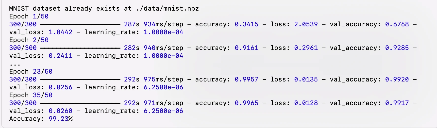
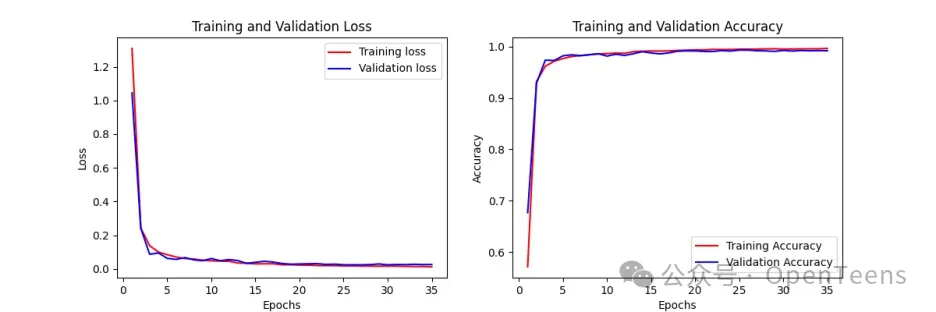
IV. Training Logs and Training Charts
Here are the logs and training curves recorded during the model training process:
V. Summary
Through this article, we successfully used the ResNet50V2 model to perform an image classification task on the MNIST dataset and built a graphical user interface (GUI) application for handwritten digit recognition. The entire process covers all steps from dataset download, preprocessing, data augmentation, model building, model training to final evaluation. The training logs and charts clearly show the model's performance during the training process.
The training curves indicate that the model learns quickly in the initial phase, with a significant drop in loss and a notable increase in accuracy. As training progresses, the model's loss and accuracy stabilize, indicating a good convergence state. Finally, the model achieved 99.23% accuracy on the test set, validating the effectiveness of using ResNet50V2 for image classification.
Additionally, we built a simple GUI application that allows users to draw handwritten digits on a canvas and predict them using the trained model. This demonstrates the potential and flexibility of deep learning in practical applications.